42 how to change labels in excel
Change legend names - Microsoft Support Select your chart in Excel, and click Design > Select Data. Click on the legend name you want to change in the Select Data Source dialog box, and click Edit. Note: You can update Legend Entries and Axis Label names from this view, and multiple Edit options might be available. Type a legend name into the Series name text box, and click OK. How to Print Avery Labels from Excel (2 Simple Methods) - ExcelDemy Step 04: Print Labels from Excel Fourthly, go to the Page Layout tab and click the Page Setup arrow at the corner. Then, select the Margins tab and adjust the page margin as shown below. Next, use CTRL + P to open the Print menu. At this point, press the No Scaling drop-down and select Fit All Columns on One Page option.
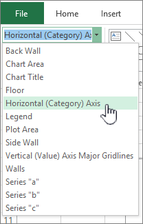
Change the display of chart axes - Microsoft Support On the Format tab, in the Current Selection group, click the arrow in the Chart Elements box, and then click the horizontal (category) axis. On the Design tab ...
How to change labels in excel
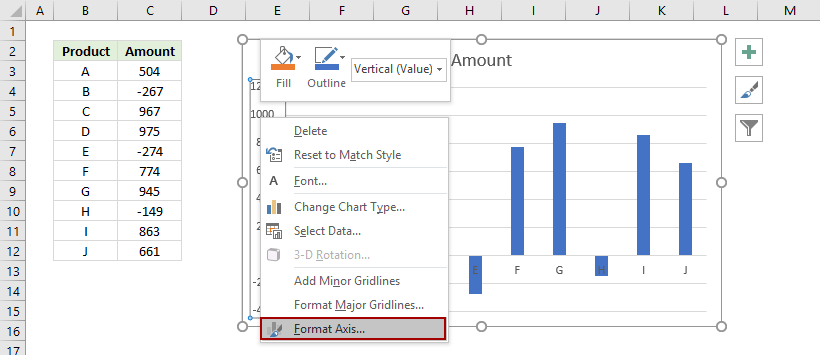
How do I change the x axis value to text in Excel? Follow the steps to change date-based X-axis intervals: Open the Excel file with your graph and select it. Right-click on the Horizontal Axis and choose Format axis. Select Axis Options. Under Units, click on the box next to Major and type in the interval number you want. Close the window, and the changes will be saved. Change axis labels in a chart in Office - Microsoft Support The chart uses text from your source data for axis labels. To change the label, you can change the text in the source data. If you don't want to change the text of the source data, you can create label text just for the chart you're working on. In addition to changing the text of labels, you can also change their appearance by adjusting formats. How to Change Excel Chart Data Labels to Custom Values? - Chandoo.org You can change data labels and point them to different cells using this little trick. First add data labels to the chart (Layout Ribbon > Data Labels) Define the new data label values in a bunch of cells, like this: Now, click on any data label. This will select "all" data labels. Now click once again.
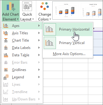
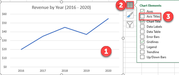
How to change labels in excel. How to rename group or row labels in Excel PivotTable? - ExtendOffice To rename Row Labels, you need to go to the Active Field textbox. 1. Click at the PivotTable, then click Analyze tab and go to the Active Field textbox. 2. Now in the Active Field textbox, the active field name is displayed, you can change it in the textbox. How to Customize Your Excel Pivot Chart Data Labels The Data Labels command on the Design tab's Add Chart Element menu in Excel allows you to label data markers with values from your pivot table. When you click the command button, Excel displays a menu with commands corresponding to locations for the data labels: None, Center, Left, Right, Above, and Below. None signifies that no data labels ... How to Add Axis Labels in Excel Charts - Step-by-Step (2022) - Spreadsheeto Left-click the Excel chart. 2. Click the plus button in the upper right corner of the chart. 3. Click Axis Titles to put a checkmark in the axis title checkbox. This will display axis titles. 4. Click the added axis title text box to write your axis label. Or you can go to the 'Chart Design' tab, and click the 'Add Chart Element' button ... Excel Chart Data Labels-Modifying Orientation - Microsoft Community Replied on September 14, 2016 In reply to PaulaAB's post on September 13, 2016 Hi Paula, You can right click on the data label part then select Format Axis. Click on the Size & Properties tab then adjust the Text Direction or Custom Angle. Thanks, Mike Report abuse 7 people found this reply helpful · Was this reply helpful? Yes No
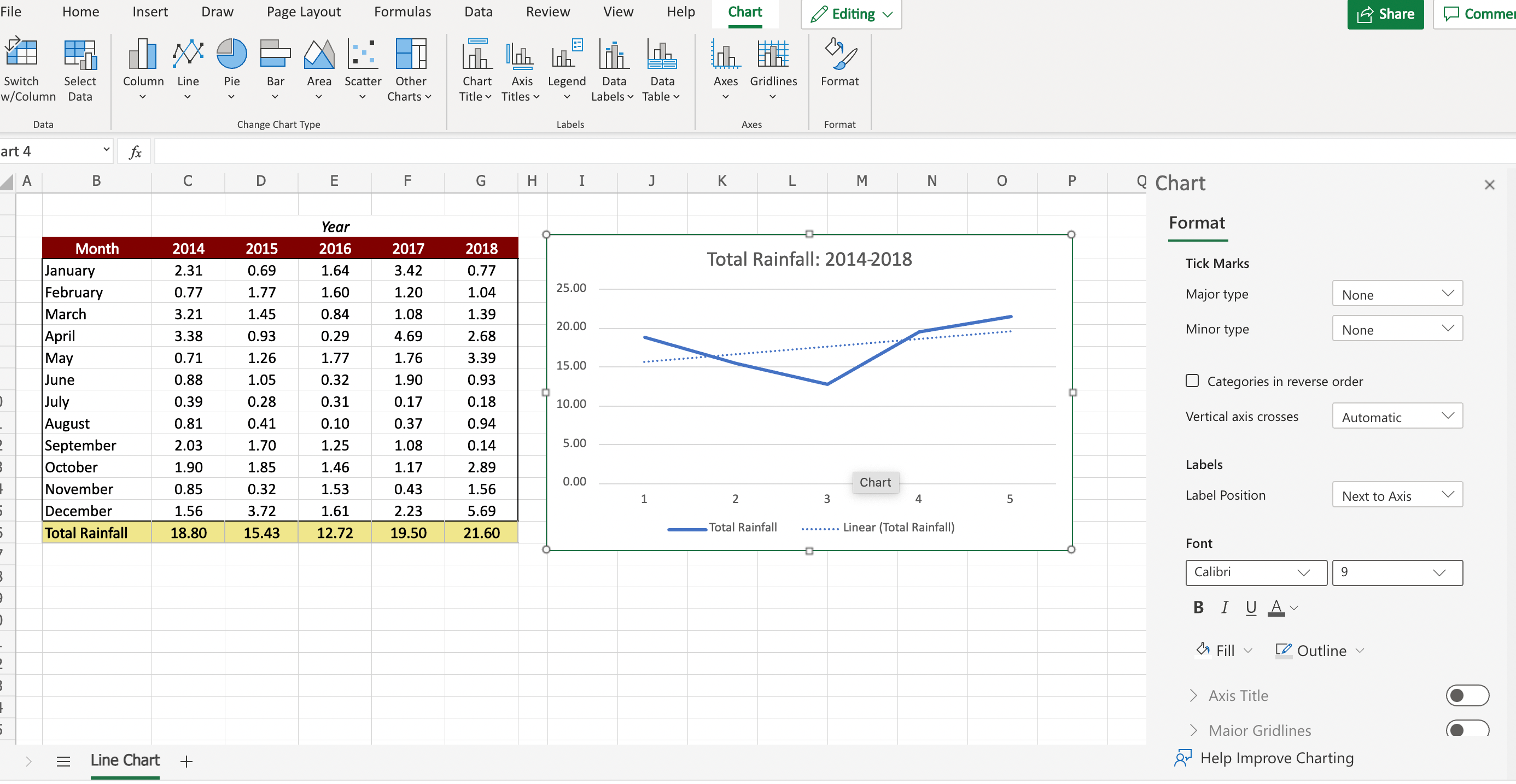
Change the format of data labels in a chart - Microsoft Support You can use leader lines to connect the labels, change the shape of the label, and resize a data label. And they're all done in the Format Data Labels task pane. To get there, after adding your data labels, select the data label to format, and then click Chart Elements > Data Labels > More Options. Excel tutorial: How to customize axis labels Instead you'll need to open up the Select Data window. Here you'll see the horizontal axis labels listed on the right. Click the edit button to access the label range. It's not obvious, but you can type arbitrary labels separated with commas in this field. So I can just enter A through F. When I click OK, the chart is updated. How to format axis labels individually in Excel - SpreadsheetWeb Double-click on the axis you want to format. Double-clicking opens the right panel where you can format your axis. Open the Axis Options section if it isn't active. You can find the number formatting selection under Number section. Select Custom item in the Category list. Type your code into the Format Code box and click Add button. How to change chart axis labels' font color and size in Excel? Right click the axis you will change labels when they are greater or less than a given value, and select the Format Axis from right-clicking menu. 2. Do one of below processes based on your Microsoft Excel version:
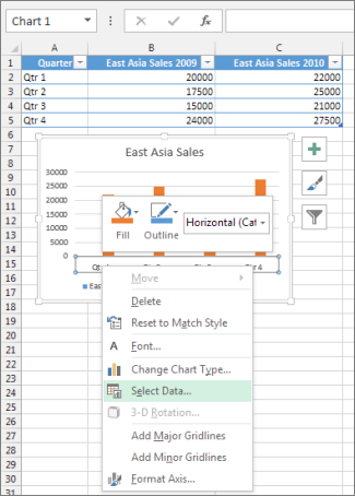
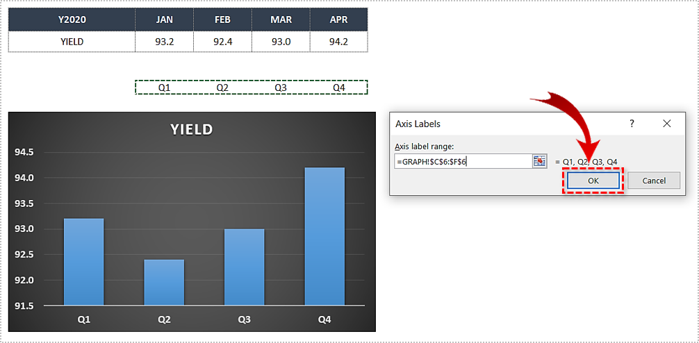
How to Print Labels from Excel - Lifewire Choose Start Mail Merge > Labels . Choose the brand in the Label Vendors box and then choose the product number, which is listed on the label package. You can also select New Label if you want to enter custom label dimensions. Click OK when you are ready to proceed. Connect the Worksheet to the Labels Change axis labels in a chart - Microsoft Support Right-click the category labels you want to change, and click Select Data. In the Horizontal (Category) Axis Labels box, click Edit. In the Axis label range box, enter the labels you want to use, separated by commas. For example, type Quarter 1,Quarter 2,Quarter 3,Quarter 4. Change the format of text and numbers in labels How to add a line in Excel graph: average line, benchmark, etc. Select the last data point on the line and add a data label to it as discussed in the previous tip. Click on the label to select it, then click inside the label box, delete the existing value and type your text: Hover over the label box until your mouse pointer changes to a four-sided arrow, and then drag the label slightly above the line: How to change the name of the column headers in Excel - Computer Hope In Microsoft Excel, click the File tab or the Office button in the upper-left corner. In the left navigation pane, click Options. In the Excel Options window, click the Advanced option in the left navigation pane. Scroll down to the Display options for this worksheet section. Uncheck the box for Show row and column headers.
X Y Scatter plot keeps changing X-Axis labels : r/excel
How to Edit Pie Chart in Excel (All Possible Modifications) Just like the chart title, you can also change the position of data labels in a pie chart. Follow the steps below to do this. 👇 Steps: Firstly, click on the chart area. Following, click on the Chart Elements icon. Subsequently, click on the rightward arrow situated on the right side of the Data Labels option.
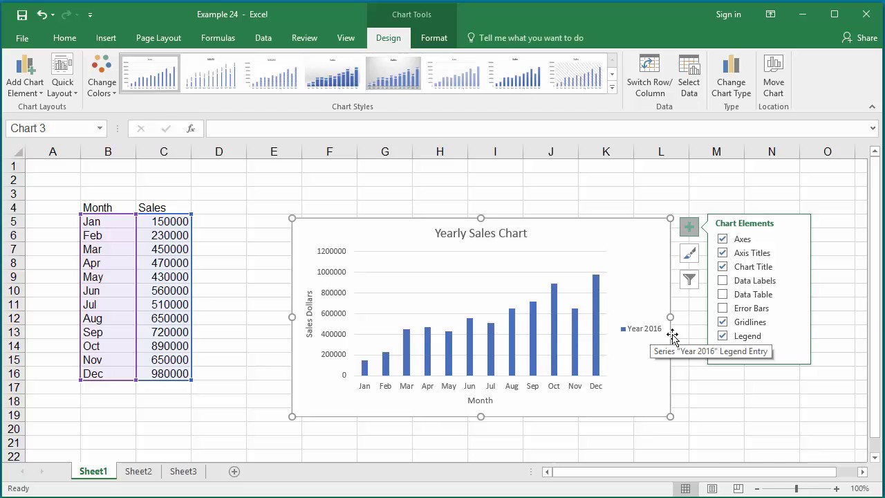
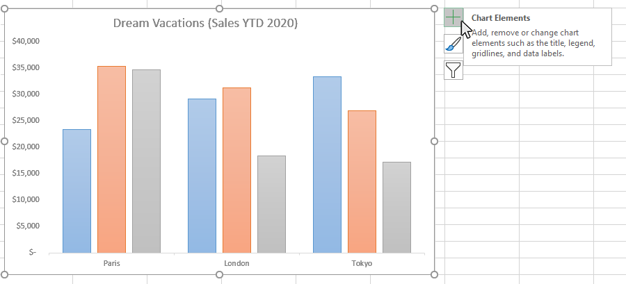
How to Change Elements of a Chart like Title, Axis Titles, Legend etc in Excel 2016
How to Rename a Data Series in Microsoft Excel - How-To Geek In the "Edit Series" box, you can begin to rename your data series labels. By default, Excel will use the column or row label, using the cell reference to determine this. Replace the cell reference with a static name of your choice. For this example, our data series labels will reflect yearly quarters (Q1 2019, Q2 2019, etc).
How to Change Font Size of Data Labels in Excel - ExcelDemy
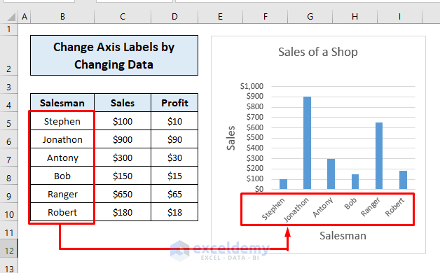
How to Change Axis Labels in Excel (3 Easy Methods) To change the label using this method, follow the steps below: Firstly, right-click the category label and click Select Data. Then, click Edit from the Horizontal (Category) Axis Labels icon. After that, assign the new labels separated with commas and click OK. Now, Your new labels are assigned.

How to Customize Your Excel Pivot Chart Data Labels - dummies
How to rotate axis labels in chart in Excel? - ExtendOffice Go to the chart and right click its axis labels you will rotate, and select the Format Axis from the context menu. 2. In the Format Axis pane in the right, click the Size & Properties button, click the Text direction box, and specify one direction from the drop down list. See screen shot below: The Best Office Productivity Tools
Change axis labels in a chart
Edit titles or data labels in a chart - support.microsoft.com In the worksheet, click the cell that contains the title or data label text that you want to change. Edit the existing contents, or type the new text or value, and then press ENTER. The changes you made automatically appear on the chart. Top of Page Reestablish the link between a title or data label and a worksheet cell
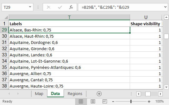
How to change the shape labels? – Example for Excel Map ...
How can I make an Excel chart refer to column or row headings? Click on the chart to select it. · Click the Chart Filters button. · Click Select Data... at the bottom right of the dialog. · In the Select Data Source dialog box ...
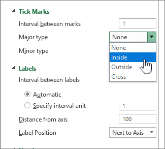
Change the display of chart axes
How to Edit Legend in Excel | Excelchat There are two ways to change the legend name: Change series name in Select Data Change legend name Change Series Name in Select Data Step 1. Right-click anywhere on the chart and click Select Data Figure 4. Change legend text through Select Data Step 2. Select the series Brand A and click Edit Figure 5. Edit Series in Excel

How to add axis titles in excel chart | WPS Office Academy
How to Print Labels From Excel - EDUCBA Step #4 - Connect Worksheet to the Labels. Now, let us connect the worksheet, which actually is containing the labels data, to these labels and then print it up. Go to Mailing tab > Select Recipients (appears under Start Mail Merge group)> Use an Existing List. A new Select Data Source window will pop up.
How to Change Horizontal Axis Labels in Excel 2010 - Solve ...
Lesson 38 - How to add DATA LABELS to charts in Excel Change colour of ... رقم الدرس : 38 . Lesson 38 - How to add DATA LABELS to charts in Excel Change colour of pie-chart segments in Excel. عرض

Add data labels and callouts to charts in Excel 365 ...
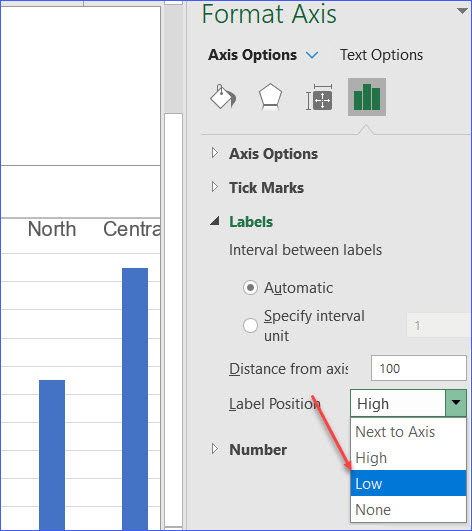
How to move Excel chart axis labels to the bottom or top - Data Cornering Move Excel chart axis labels to the bottom in 2 easy steps. Select horizontal axis labels and press Ctrl + 1 to open the formatting pane. Open the Labels section and choose label position " Low ". Here is the result with Excel chart axis labels at the bottom. Now it is possible to clearly evaluate the dynamics of the series and see axis labels.

Format Data Labels in Excel- Instructions - TeachUcomp, Inc.
Data Labels in Excel Pivot Chart (Detailed Analysis) Next open Format Data Labels by pressing the More options in the Data Labels. Then on the side panel, click on the Value From Cells. Next, in the dialog box, Select D5:D11, and click OK. Right after clicking OK, you will notice that there are percentage signs showing on top of the columns. 4. Changing Appearance of Pivot Chart Labels
Change the display of chart axes
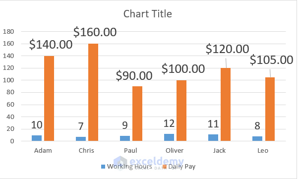
How to add data labels from different column in an Excel chart? Please do as follows: 1. Right click the data series in the chart, and select Add Data Labels > Add Data Labels from the context menu to add data labels. 2. Right click the data series, and select Format Data Labels from the context menu. 3.

Custom data labels in a chart
How to Change Excel Chart Data Labels to Custom Values? - Chandoo.org You can change data labels and point them to different cells using this little trick. First add data labels to the chart (Layout Ribbon > Data Labels) Define the new data label values in a bunch of cells, like this: Now, click on any data label. This will select "all" data labels. Now click once again.

charts - How do I create custom axes in Excel? - Super User
Change axis labels in a chart in Office - Microsoft Support The chart uses text from your source data for axis labels. To change the label, you can change the text in the source data. If you don't want to change the text of the source data, you can create label text just for the chart you're working on. In addition to changing the text of labels, you can also change their appearance by adjusting formats.

How to Change Horizontal Axis Labels in Excel | How to Create Custom X Axis Labels
How do I change the x axis value to text in Excel? Follow the steps to change date-based X-axis intervals: Open the Excel file with your graph and select it. Right-click on the Horizontal Axis and choose Format axis. Select Axis Options. Under Units, click on the box next to Major and type in the interval number you want. Close the window, and the changes will be saved.

Change the format of data labels in a chart

Change Horizontal Axis Values in Excel 2016 - AbsentData

charts - How to change interval between labels in Excel 2013 ...
How to Move X Axis Labels from Top to Bottom - ExcelNotes

Change color of data label placed, using the 'best fit ...
Change the display of chart axes

Change the format of data labels in a chart

How to Change Axis Labels in Excel - TechObservatory

Custom Excel Chart Label Positions • My Online Training Hub

How to Change Axis Values in Excel | Excelchat
How to Add Axis Labels to a Chart in Excel - Business ...

Changing Axis Labels in Excel 2016 for Mac - Microsoft Community

how to add data labels into Excel graphs — storytelling with data

Custom Data Labels with Colors and Symbols in Excel Charts ...
Don't know how to change horizontal axis labels on Mac OS ...

Change the format of data labels in a chart

Excel charts: add title, customize chart axis, legend and ...

charts - Can't edit horizontal (catgegory) axis labels in ...

Change axis labels in a chart
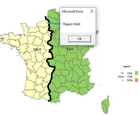
How to change the shape labels? – Example for Excel Map ...

Change the format of data labels in a chart
How to move chart X axis below negative values/zero/bottom in ...
How to add Axis Labels (X & Y) in Excel & Google Sheets ...

How to Change Axis Labels in Excel (3 Easy Methods) - ExcelDemy
How to Change the X-Axis in Excel
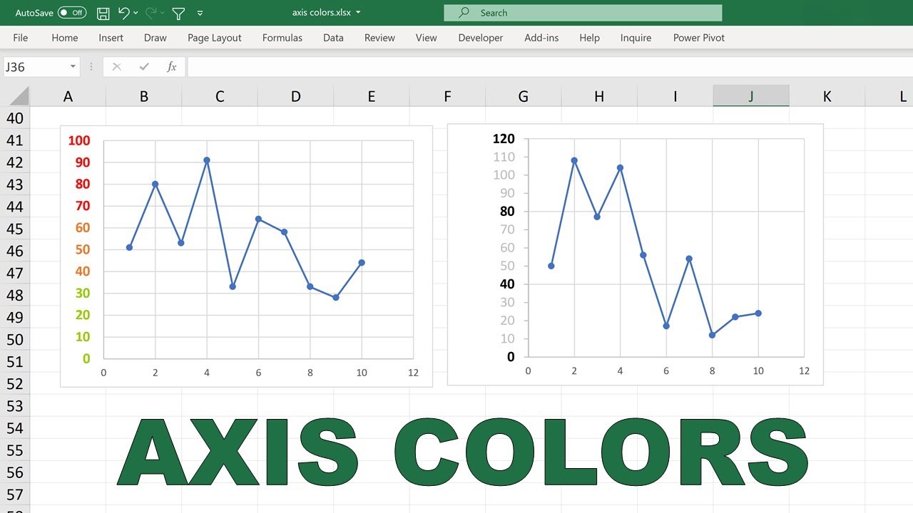
How to make the font of the axis labels different colors in an excel chart
How to Change Axis Labels in Excel (3 Easy Methods) - ExcelDemy
Post a Comment for "42 how to change labels in excel"