45 add custom data labels to excel chart
How to format axis labels individually in Excel - SpreadsheetWeb Double-click on the axis you want to format. Double-clicking opens the right panel where you can format your axis. Open the Axis Options section if it isn't active. You can find the number formatting selection under Number section. Select Custom item in the Category list. Type your code into the Format Code box and click Add button. How to set multiple series labels at once - Microsoft Tech Community If the range containing the series names is adjacent to the series values, try the following: Click anywhere in the chart. On the Chart Design tab of the ribbon, in the Data group, click Select Data. Click in the 'Chart data range' box. Select the range containing both the series names and the series values. Click OK.
support.microsoft.com › en-us › officeAdd or remove data labels in a chart - support.microsoft.com Depending on what you want to highlight on a chart, you can add labels to one series, all the series (the whole chart), or one data point. Add data labels. You can add data labels to show the data point values from the Excel sheet in the chart. This step applies to Word for Mac only: On the View menu, click Print Layout.
Add custom data labels to excel chart
How to Add Leader Lines in Excel? - GeeksforGeeks Step 2: Go to Insert Tab and select Recommended Charts. A dialogue box name Insert Chart appears. Step 3: Click on All Charts and select Line. Click Ok. Step 4: A line chart is embedded in the worksheet. Step 5: Go to Chart Design Tab and select Add Chart Element . Step 6: Hover on the Data Labels option. Click on More Data Label Options …. DataLabels.Separator property (Excel) | Microsoft Docs Example This example sets the data label separator for the first series on the first chart to a semicolon. This example assumes that a chart exists on the active worksheet. VB Copy Sub ChangeSeparator () ActiveSheet.ChartObjects (1).Chart.SeriesCollection (1) _ .DataLabels.Separator = ";" End Sub Support and feedback › how-to-create-excel-pie-chartsHow to Make a Pie Chart in Excel & Add Rich Data Labels to ... Sep 08, 2022 · In this article, we are going to see a detailed description of how to make a pie chart in excel. One can easily create a pie chart and add rich data labels, to one’s pie chart in Excel. So, let’s see how to effectively use a pie chart and add rich data labels to your chart, in order to present data, using a simple tennis related example.
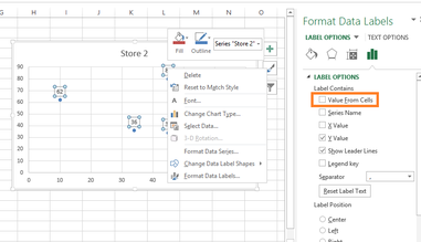
Add custom data labels to excel chart. › 509290 › how-to-use-cell-valuesHow to Use Cell Values for Excel Chart Labels - How-To Geek Mar 12, 2020 · Select the chart, choose the “Chart Elements” option, click the “Data Labels” arrow, and then “More Options.” Uncheck the “Value” box and check the “Value From Cells” box. Select cells C2:C6 to use for the data label range and then click the “OK” button. peltiertech.com › add-horizontal-line-to-excel-chartAdd a Horizontal Line to an Excel Chart - Peltier Tech Sep 11, 2018 · Copy the data, select the chart, and Paste Special to add the data as a new series. Right click on the added series, and change its chart type to XY Scatter With Straight Lines And Markers (again, the markers are temporary). How to: Display and Format Data Labels - DevExpress Add Data Labels to the Chart Specify the Position of Data Labels Apply Number Format to Data Labels Create a Custom Label Entry Add Data Labels to the Chart Basic settings that specify the contents, position and appearance of data labels in the chart are defined by the DataLabelOptions object, accessed by the ChartView.DataLabels property. How to Add Data Table in an Excel Chart (4 Quick Methods) 4 Methods for Data Table in Excel Chart 1. Add Data Table From Chart Design Tab in Excel 1.1. Show Data Table Using 'Quick Layout' Option 1.2. Use the 'Add Chart Element' Option to Show Data Tables 2. Show/Hide Data Table by Clicking the Plus (+) Sign of Excel Chart 3. Add Extra Data Series to Data Table but Not in Chart 4.
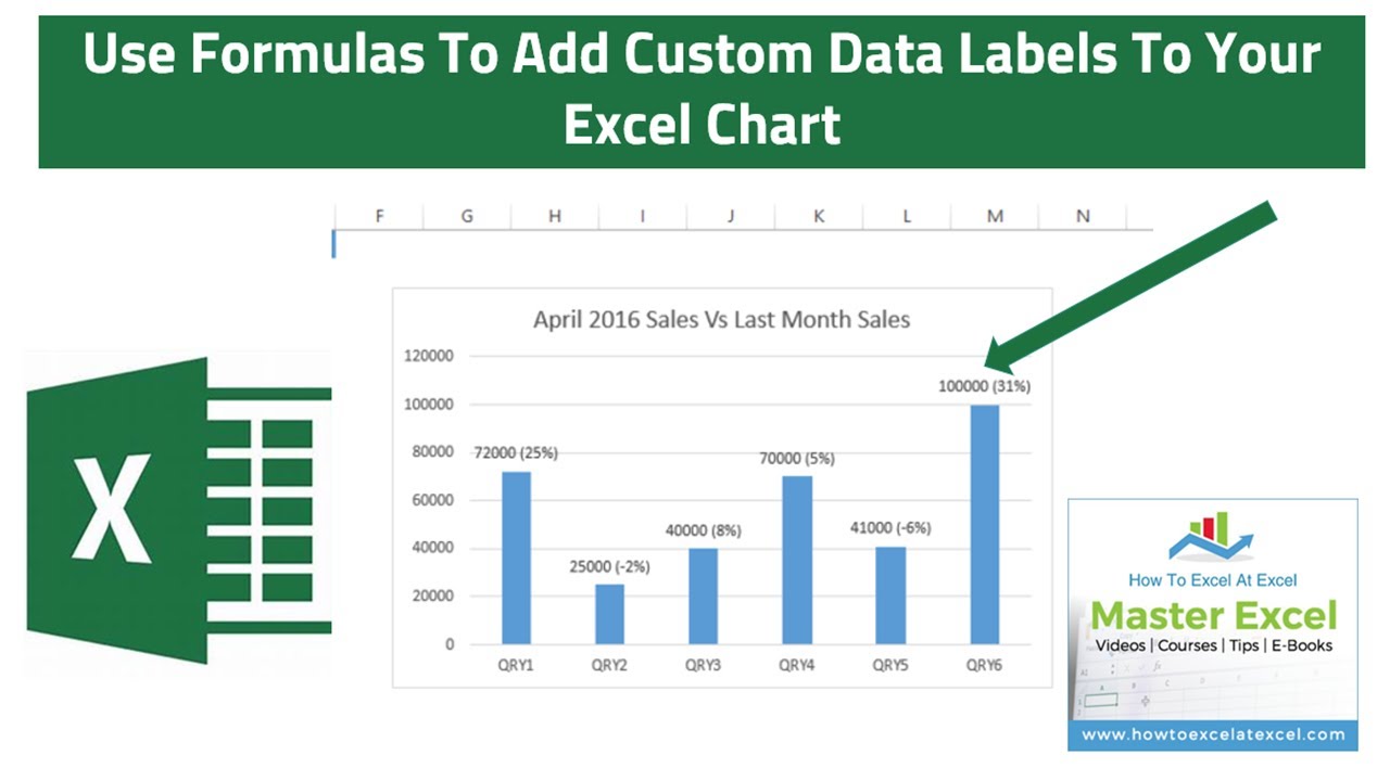
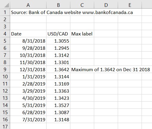
How to Show Percentage in Bar Chart in Excel (3 Handy Methods) - ExcelDemy 📌 Step 04: Include New Series for Data Labels Fourthly, select the chart and right-click on the mouse to go to the Select Data option. Next, click the Add button to include a new series. Now, enter the name Max 1, and select the G5:G10 cells as shown below. Similarly, add the series Max 2, and again choose the G5:G10 cells. Custom Chart Data Labels In Excel With Formulas - How To Excel At Excel Follow the steps below to create the custom data labels. Select the chart label you want to change. In the formula-bar hit = (equals), select the cell reference containing your chart label's data. In this case, the first label is in cell E2. Finally, repeat for all your chart laebls. chandoo.org › wp › change-data-labels-in-chartsHow to Change Excel Chart Data Labels to Custom Values? May 05, 2010 · First add data labels to the chart (Layout Ribbon > Data Labels) Define the new data label values in a bunch of cells, like this: Now, click on any data label. This will select “all” data labels. Now click once again. At this point excel will select only one data label. How to Create a Mekko Chart (Marimekko) in Excel - Quick Guide Here are the steps to create a Mekko chart: #1: Set up a helper table and add data. #2: Append the helper table with zeros. #3: Apply a custom number format. #4: Calculate and add segment values. #5: Set up the horizontal axis values. #6: Calculate midpoints. #7: Add labels for rows and columns.
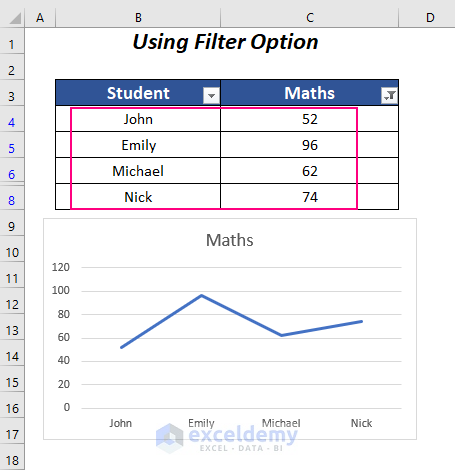
Radial Bar Chart in Excel - Quick Guide - ExcelKid Prepare the labels for the radial bar chart. First, create a helper column for the data labels on column E. ... UDT is a professional Excel data visualization and chart add-in containing many special chart functions. ... But the work is worth it; we get a custom, easy-to-read graph. So if you need to build a sales comparison, we strongly ... How to Add Axis Titles in a Microsoft Excel Chart - How-To Geek Select the chart and go to the Chart Design tab. Click the Add Chart Element drop-down arrow, move your cursor to Axis Titles, and deselect "Primary Horizontal," "Primary Vertical," or both. In Excel on Windows, you can also click the Chart Elements icon and uncheck the box for Axis Titles to remove them both. If you want to keep one ... How to Apply a Filter to a Chart in Microsoft Excel - How-To Geek Select the data for your chart, not the chart itself. Go to the Home tab, click the Sort & Filter drop-down arrow in the ribbon, and choose "Filter." Click the arrow at the top of the column for the chart data you want to filter. Use the Filter section of the pop-up box to filter by color, condition, or value. › charts › dynamic-chart-dataCreate Dynamic Chart Data Labels with Slicers - Excel Campus Feb 10, 2016 · This is because Excel 2010 does not contain the Value from Cells feature. Jon Peltier has a great article with some workarounds for applying custom data labels. This includes using the XY Chart Labeler Add-in, which is a free download for Windows or Mac. Step 6: Setup the Pivot Table and Slicer. The final step is to make the data labels ...
Add / Move Data Labels in Charts – Excel & Google Sheets ...
Excel Charts with Shapes for Infographics - My Online Training Hub Tip: add data labels and remove the gridlines and vertical axis. Caution: the shape will be stretched to fit the different column sizes. In the chart above it's barely noticeable, however see the next step if this is an issue. ... Custom Excel Chart Label Positions using a dummy or ghost series to force the label position neatly above the ...
How can I format individual data points in Google Sheets ...
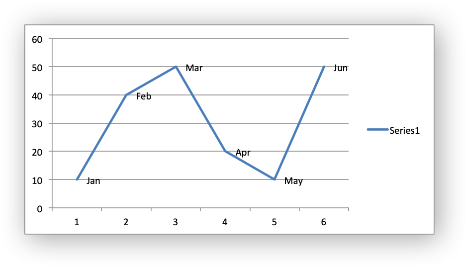
Label line chart series - Get Digital Help Double press with left mouse button on the cell that contains the data label. Put the prompt between the words. Press Alt + Enter. Press Enter. Back to top 3. Align data labels If you want the labels to be aligned to the left simply select the data label. Go to tab "Home" on the ribbon. Press with left mouse button on the "Align Left" button.
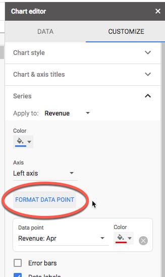
How can I format individual data points in Google Sheets ...
How to add text labels on Excel scatter chart axis - Data Cornering 3. Add dummy series to the scatter plot and add data labels. 4. Select recently added labels and press Ctrl + 1 to edit them. Add custom data labels from the column "X axis labels". Use "Values from Cells" like in this other post and remove values related to the actual dummy series. Change the label position below data points.

Data Labels | FlexChart | ComponentOne
How to: Display and Format Data Labels - DevExpress Add Data Labels to the Chart Specify the Position of Data Labels Apply Number Format to Data Labels Create a Custom Label Entry Add Data Labels to the Chart Basic settings that specify the contents, position and appearance of data labels in the chart are defined by the DataLabelOptions object, accessed by the ChartView.DataLabels property.

How to Customize for a GREAT-Looking Excel Chart
Modifying Axis Scale Labels (Microsoft Excel) - tips Follow these steps: Create your chart as you normally would. Double-click the axis you want to scale. You should see the Format Axis dialog box. (If double-clicking doesn't work, right-click the axis and choose Format Axis from the resulting Context menu.) Make sure the Number tab is displayed. (See Figure 1.)

How to show data labels in PowerPoint and place them ...
How to add data labels in excel to graph or chart (Step-by-Step) Add data labels to a chart 1. Select a data series or a graph. After picking the series, click the data point you want to label. 2. Click Add Chart Element Chart Elements button > Data Labels in the upper right corner, close to the chart. 3. Click the arrow and select an option to modify the location. 4.

how to add data labels into Excel graphs — storytelling with data
How to Create and Customize a Treemap Chart in Microsoft Excel Select the data for the chart and head to the Insert tab. Click the "Hierarchy" drop-down arrow and select "Treemap." The chart will immediately display in your spreadsheet. And you can see how the rectangles are grouped within their categories along with how the sizes are determined.

Using the CONCAT function to create custom data labels for an ...
DataLabel object (Excel) | Microsoft Docs Copy With Charts ("chart1") With .SeriesCollection (1).Points (2) .HasDataLabel = True .DataLabel.Text = "Saturday" End With End With On a trendline, the DataLabel property returns the text shown with the trendline. This can be the equation, the R-squared value, or both (if both are showing).
Create Custom Data Labels. Excel Charting.
How To Add a Legend to a Chart in Excel (2 Methods, FAQs) Select "Chart Design" in the command ribbon: This opens additional options you can select to change your chart. Click "Add Chart Element": This option is on the far left of the command ribbon and opens a drop-down menu when you select it. Select "Legend": This opens an additional menu, which enables you to select the location for your legend.

Add or remove data labels in a chart
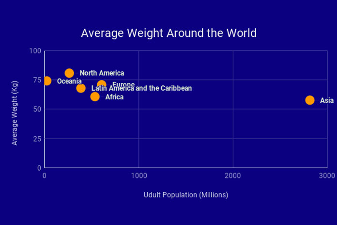
Bubble Chart in Excel - Step-by-step Guide #7: Add values and comment labels. Select the "Sales" series, right-click, and choose "Add Labels". You will see only zeros, but no worry! Right-click on the labels; the "Format Data Labels" will appear. Under the "Label Options", check the "Values From Cells" checkbox. Select the B3:B25 range.
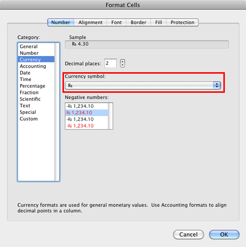
Format Number Options for Chart Data Labels in Excel 2011 for Mac
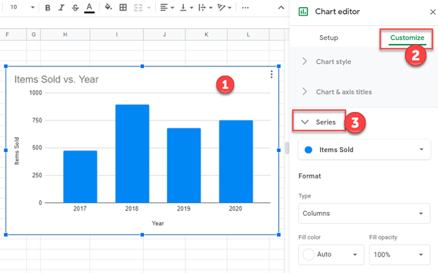
› charts › add-data-pointAdd Data Points to Existing Chart – Excel & Google Sheets Similar to Excel, create a line graph based on the first two columns (Months & Items Sold) Right click on graph; Select Data Range . 3. Select Add Series. 4. Click box for Select a Data Range. 5. Highlight new column and click OK. Final Graph with Single Data Point

microsoft excel - Adding data label only to the last value ...
Adding Data Labels to Your Chart (Microsoft Excel) - ExcelTips (ribbon) To add data labels in Excel 2013 or later versions, follow these steps: Activate the chart by clicking on it, if necessary. Make sure the Design tab of the ribbon is displayed. (This will appear when the chart is selected.) Click the Add Chart Element drop-down list. Select the Data Labels tool.
Google Sheets - Add Labels to Data Points in Scatter Chart
Use defined names to automatically update a chart range - Office Select cells A1:B4. On the Insert tab, click a chart, and then click a chart type.. Click the Design tab, click the Select Data in the Data group.. Under Legend Entries (Series), click Edit.. In the Series values box, type =Sheet1!Sales, and then click OK.. Under Horizontal (Category) Axis Labels, click Edit.. In the Axis label range box, type =Sheet1!Date, and then click OK.

Change the format of data labels in a chart
How to Print Labels from Excel - Lifewire Choose Start Mail Merge > Labels . Choose the brand in the Label Vendors box and then choose the product number, which is listed on the label package. You can also select New Label if you want to enter custom label dimensions. Click OK when you are ready to proceed. Connect the Worksheet to the Labels

Add or remove data labels in a chart
DataLabels object (Excel) | Microsoft Docs Use the DataLabels method of the Series object to return the DataLabels collection. The following example sets the number format for data labels on series one on chart sheet one. VB Copy With Charts (1).SeriesCollection (1) .HasDataLabels = True .DataLabels.NumberFormat = "##.##" End With

Display Customized Data Labels on Charts & Graphs
How to Display Percentage in an Excel Graph (3 Methods) Then go to the More Options via the right arrow beside the Data Labels. Select Chart on the Format Data Labels dialog box. Uncheck the Value option. Check the Value From Cells option. Then you have to select cell ranges to extract percentage values. For this purpose, create a column called Percentage using the following formula: =E5/C5

How to add or move data labels in Excel chart?
› how-to-create-excel-pie-chartsHow to Make a Pie Chart in Excel & Add Rich Data Labels to ... Sep 08, 2022 · In this article, we are going to see a detailed description of how to make a pie chart in excel. One can easily create a pie chart and add rich data labels, to one’s pie chart in Excel. So, let’s see how to effectively use a pie chart and add rich data labels to your chart, in order to present data, using a simple tennis related example.
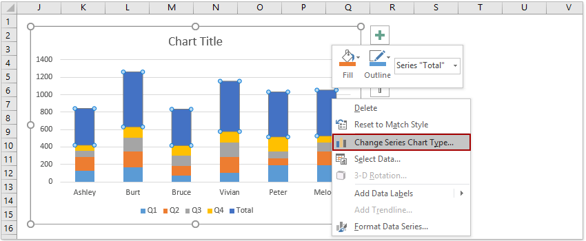
How to add total labels to stacked column chart in Excel?
DataLabels.Separator property (Excel) | Microsoft Docs Example This example sets the data label separator for the first series on the first chart to a semicolon. This example assumes that a chart exists on the active worksheet. VB Copy Sub ChangeSeparator () ActiveSheet.ChartObjects (1).Chart.SeriesCollection (1) _ .DataLabels.Separator = ";" End Sub Support and feedback
Help Online - Quick Help - FAQ-133 How do I label the data ...
How to Add Leader Lines in Excel? - GeeksforGeeks Step 2: Go to Insert Tab and select Recommended Charts. A dialogue box name Insert Chart appears. Step 3: Click on All Charts and select Line. Click Ok. Step 4: A line chart is embedded in the worksheet. Step 5: Go to Chart Design Tab and select Add Chart Element . Step 6: Hover on the Data Labels option. Click on More Data Label Options ….

How to Add Data Labels to an Excel 2010 Chart - dummies
Working with Charts — XlsxWriter Documentation

How to Create a Pie Chart in Excel | Smartsheet

Dynamically Label Excel Chart Series Lines • My Online ...

How to Add Data Labels to your Excel Chart in Excel 2013

Add Labels ON Your Bars
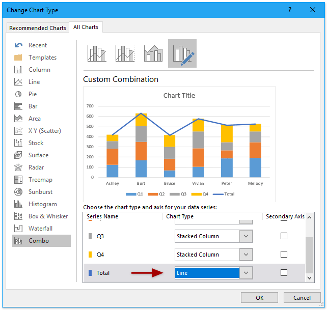
How to add total labels to stacked column chart in Excel?
Add Custom Labels to x-y Scatter plot in Excel - DataScience ...
Help Online - Quick Help - FAQ-133 How do I label the data ...

Adding rich data labels to charts in Excel 2013 | Microsoft ...

How to create Custom Data Labels in Excel Charts

excel - How to show series-Legend label name in data labels ...
Using the CONCAT function to create custom data labels for an ...

Apply Custom Data Labels to Charted Points - Peltier Tech
How to Remove Zero Data Labels in Excel Graph (3 Easy Ways)
How to Place Labels Directly Through Your Line Graph in ...

Custom data labels in a chart
vba - Excel XY Chart (Scatter plot) Data Label No Overlap ...

How to Change Excel Chart Data Labels to Custom Values?
Custom Excel Chart Label Positions • My Online Training Hub

Excel Custom Chart Labels • My Online Training Hub
How-to Add Custom Labels that Dynamically Change in Excel ...

How to Place Labels Directly Through Your Line Graph in ...

Apply Custom Data Labels to Charted Points - Peltier Tech
How to Create a Timeline Chart in Excel - Automate Excel

Improve your X Y Scatter Chart with custom data labels
Post a Comment for "45 add custom data labels to excel chart"