42 how to change excel chart data labels to custom values

excel - Formatting chart data labels with VBA - Stack Overflow Select Case seriesfmt Case "int" Cht.SeriesCollection (i).DataLabels.NumberFormat = "#" Case "#,#" Cht.SeriesCollection (i).DataLabels.NumberFormat = "#,###" Case "%" Cht.SeriesCollection (i).DataLabels.NumberFormat = "#.0%" End Select End If Next i Finally the real problem here: what goes in between. I cannot retrieve the series format! How to create Custom Data Labels in Excel Charts Two ways to do it. Click on the Plus sign next to the chart and choose the Data Labels option. We do NOT want the data to be shown. To customize it, click on the arrow next to Data Labels and choose More Options … Unselect the Value option and select the Value from Cells option. Choose the third column (without the heading) as the range.

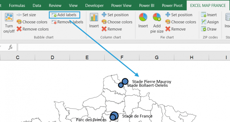
Add data labels and callouts to charts in Excel 365 | EasyTweaks.com Step #2: When you select the "Add Labels" option, all the different portions of the chart will automatically take on the corresponding values in the table that you used to generate the chart.The values in your chat labels are dynamic and will automatically change when the source value in the table changes. Step #3: Format the data labels.. Excel also gives you the option of formatting the ...

How to change excel chart data labels to custom values

How to Change Excel Chart Data Labels to Custom Values? First add data labels to the chart (Layout Ribbon > Data Labels) Define the new data label values in a bunch of cells, like this: Now, click on any data label. This will select "all" data labels. Now click once again. At this point excel will select only one data label. Custom Chart Data Labels In Excel With Formulas Follow the steps below to create the custom data labels. Select the chart label you want to change. In the formula-bar hit = (equals), select the cell reference containing your chart label's data. In this case, the first label is in cell E2. Finally, repeat for all your chart laebls. Edit titles or data labels in a chart - support.microsoft.com The first click selects the data labels for the whole data series, and the second click selects the individual data label. Right-click the data label, and then click Format Data Label or Format Data Labels. Click Label Options if it's not selected, and then select the Reset Label Text check box. Top of Page

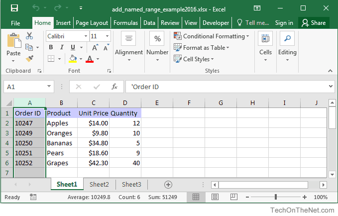
How to change excel chart data labels to custom values. How to Use Cell Values for Excel Chart Labels Select the chart, choose the "Chart Elements" option, click the "Data Labels" arrow, and then "More Options." Uncheck the "Value" box and check the "Value From Cells" box. Select cells C2:C6 to use for the data label range and then click the "OK" button. The values from these cells are now used for the chart data labels. Custom Data Labels with Colors and Symbols in Excel Charts - [How To] To apply custom format on data labels inside charts via custom number formatting, the data labels must be based on values. You have several options like series name, value from cells, category name. But it has to be values otherwise colors won't appear. Symbols issue is quite beyond me. Create Dynamic Chart Data Labels with Slicers - Excel Campus You basically need to select a label series, then press the Value from Cells button in the Format Data Labels menu. Then select the range that contains the metrics for that series. Click to Enlarge Repeat this step for each series in the chart. If you are using Excel 2010 or earlier the chart will look like the following when you open the file. Excel charts: add title, customize chart axis, legend and data labels Select the chart and go to the Chart Tools tabs ( Design and Format) on the Excel ribbon. Right-click the chart element you would like to customize, and choose the corresponding item from the context menu. Use the chart customization buttons that appear in the top right corner of your Excel graph when you click on it.

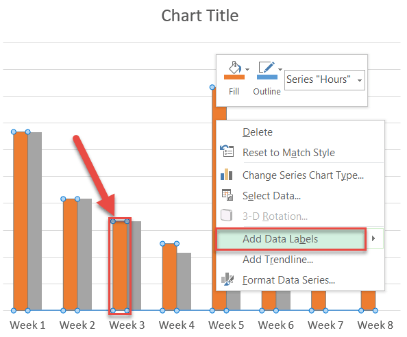
How to add and customize chart data labels - Get Digital Help Double press with left mouse button on with left mouse button on a data label series to open the settings pane. Go to tab "Label Options" see image to the right. The checkboxes let you select what values you want to use as data labels. Value from cells - Lets you select a cell range that contains the values you want to use. Modify Excel Chart Data Range | CustomGuide Select the chart Click the Design tab. Click the Select Data button. Select the series you want to change under Legend Entries (Series). Click the Edit button. Type the label you want to use for the series in the Series name field. Click OK. Click OK again. The name is updated in the chart, but the worksheet data remains unchanged. Apply Custom Data Labels to Charted Points - Peltier Tech Double click on the label to highlight the text of the label, or just click once to insert the cursor into the existing text. Type the text you want to display in the label, and press the Enter key. Repeat for all of your custom data labels. This could get tedious, and you run the risk of typing the wrong text for the wrong label (I initially ... Custom data labels in a chart - Get Digital Help Press with mouse on "Add Data Labels". Press with mouse on Add Data Labels". Double press with left mouse button on any data label to expand the "Format Data Series" pane. Enable checkbox "Value from cells". A small dialog box prompts for a cell range containing the values you want to use a s data labels.

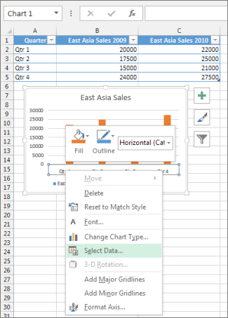
Using the CONCAT function to create custom data labels for an Excel chart Use the chart skittle (the "+" sign to the right of the chart) to select Data Labels and select More Options to display the Data Labels task pane. Check the Value From Cells checkbox and select the cells containing the custom labels, cells C5 to C16 in this example. It is important to select the entire range because the label can move based ... Is there a way to change the order of Data Labels? Please try to double click the the part of the label value, and choose the one you want to show to change the order. Thanks, Rena ----------------------- * Beware of scammers posting fake support numbers here. * Once complete conversation about this topic, kindly Mark and Vote any replies to benefit others reading this thread. Report abuse Add a DATA LABEL to ONE POINT on a chart in Excel All the data points will be highlighted. Click again on the single point that you want to add a data label to. Right-click and select ' Add data label '. This is the key step! Right-click again on the data point itself (not the label) and select ' Format data label '. You can now configure the label as required — select the content of ... How to Change Axis Values in Excel - Excelchat Right-click on the chart and choose Select Data Click on the button Switch Row/Column and press OK Figure 11. Switch x and y axis As a result, switches x and y axis and each store represent one series: Figure 12. How to swap x and y axis The chart will have more logic if we track store values per years.

Change Series Name Excel Mac

How to change chart axis labels' font color and size in Excel? Sometimes, you may want to change labels' font color by positive/negative/ in an axis in chart. You can get it done with conditional formatting easily as follows: 1. Right click the axis you will change labels by positive/negative/0, and select the Format Axis from right-clicking menu. 2.

Change axis labels in a chart - Office Support

editing Excel histogram chart horizontal labels - Microsoft Community editing Excel histogram chart horizontal labels. I have a chart of continuous data values running from 1-7. The horizontal axis values show as intervals [1,2] [2,3] and so on. I want the values to show as 1 2 3 etc. I have tried inserting a column of the values 1-7 alongside the data and selecting that as axis values; copying the data to a new ...

How to geocode customer addresses and show them on an Excel bubble chart? – Maps for Excel ...

Change the format of data labels in a chart To get there, after adding your data labels, select the data label to format, and then click Chart Elements > Data Labels > More Options. To go to the appropriate area, click one of the four icons ( Fill & Line, Effects, Size & Properties ( Layout & Properties in Outlook or Word), or Label Options) shown here.

Excel chart with a single x-axis but two different ranges (combining horizontal clustered bar ...

Use custom formats in an Excel chart's axis and data labels Right-click the Axis area and choose Format Axis from the context menu. If you don't see Format Axis, right-click another spot. Choose Number in the left pane. (In Excel 2003, click the Number ...

Improve your X Y Scatter Chart with custom data labels

excel - How do I update the data label of a chart? - Stack Overflow Select the data label Then, place your cursor in Excel's Formula Bar, and enter the formula like ='Sheet2'!$C$3. Now, that data label is associated by the formula, to the cell C3, which contains the desired data label that we built above. Repeat as needed. Note: The sheet name is required in this formula.

How to Create a Mekko/Marimekko Chart in Excel - Automate Excel

How to Customize Your Excel Pivot Chart Data Labels If you want to label data markers with a category name, select the Category Name check box. To label the data markers with the underlying value, select the Value check box. In Excel 2007 and Excel 2010, the Data Labels command appears on the Layout tab. Also, the More Data Labels Options command displays a dialog box rather than a pane.

How to Create a Timeline Chart in Excel - Automate Excel

Excel tutorial: How to customize axis labels Instead you'll need to open up the Select Data window. Here you'll see the horizontal axis labels listed on the right. Click the edit button to access the label range. It's not obvious, but you can type arbitrary labels separated with commas in this field. So I can just enter A through F. When I click OK, the chart is updated.

34 Axis Label Range - Labels Design Ideas 2020

Custom Excel Chart Label Positions - My Online Training Hub Custom Excel Chart Label Positions - Setup. The source data table has an extra column for the 'Label' which calculates the maximum of the Actual and Target: The formatting of the Label series is set to 'No fill' and 'No line' making it invisible in the chart, hence the name 'ghost series': The Label Series uses the 'Value ...

Share :